44 data labels excel 2013
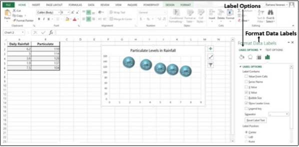
Adding Data Labels to Your Chart (Microsoft Excel) To add data labels in Excel 2013 or Excel 2016, follow these steps: Activate the chart by clicking on it, if necessary. Make sure the Design tab of the ribbon is displayed. (This will appear when the chart is selected.) Click the Add Chart Element drop-down list. Select the Data Labels tool. Data Labels auto fill [SOLVED] - Excel Help Forum On excel 2013 I was able to do it by highlighting the data labels, clicking format and choose from value and it would set them up perfectly But at work they use excel 2007 and all the data labels turned to [Cell Range] I know you can click each data label individually and type "=" and then click on the cell you want to set it to but I've got ...
Values From Cell: Missing Data Labels Option in Excel 2013 ... A couple articles refer to formatting data labels and values to have it pull what you want. I have a feeling they used a 3rd party ad-in like tech-cell or some such and because I don't have the add in its not happy. Im following the blog reference here: Adding rich data labels to charts in Excel 2013 - Office Blogs

Data labels excel 2013
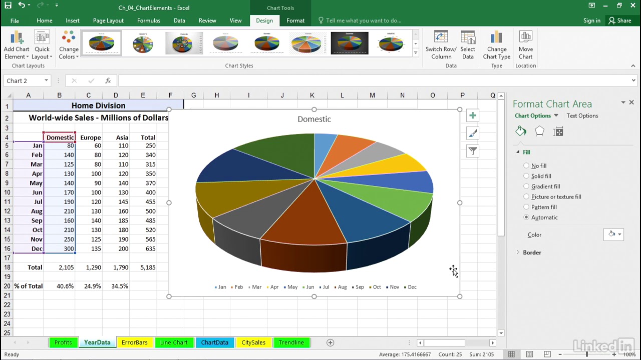
Excel Tips n Tricks -Tip 8 (Applying Chart Data Labels ... Click on the plus symbol, the first icon, and check "Data Labels". Now you will see them added to your chart. You can also click on the right arrow on "Data Labels" and select where you want the data labels to be aligned, in other words center, right, top, bottom and so on. Picture 4 4. I modified the chart and axis titles to look good. How to Create and Label a Pie Chart in Excel 2013 : 8 ... Step 8: Label the Chart. Check the "Data Labels" square and the labels will appear on the pie chart. Congratulations, you have successfully created a labeled pie chart. Note: If you want to re-position the labels, hover your cursor over the "Data Labels" option and click on the small, black triangle that appears next to it. How to Add Data Labels in Excel - Excelchat | Excelchat How to Add Data Labels In Excel 2013 And Later Versions In Excel 2013 and the later versions we need to do the followings; Click anywhere in the chart area to display the Chart Elements button Figure 5. Chart Elements Button Click the Chart Elements button > Select the Data Labels, then click the Arrow to choose the data labels position. Figure 6.
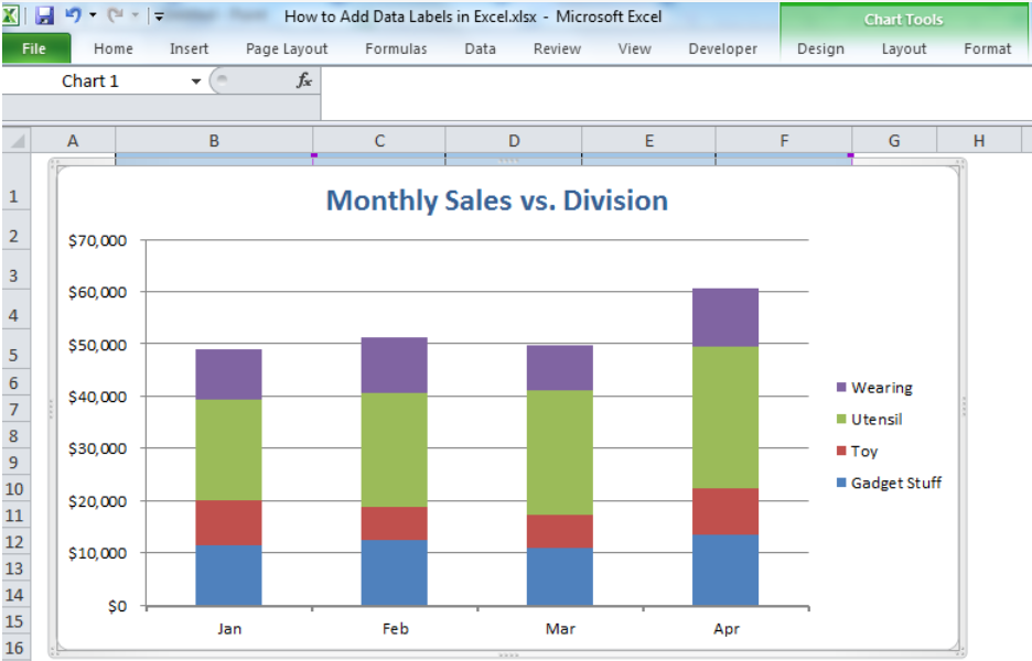
Data labels excel 2013. How to Print Labels From Excel? | Steps to Print Labels ... Step #1 - Add Data into Excel. Create a new excel file with the name "Print Labels from Excel" and open it. Add the details to that sheet. As we want to create mailing labels, make sure each column is dedicated to each label. Ex. Excel 2013 Graphs automatically aligning data labels to ... Excel 2013 Graphs automatically aligning data labels to end of bar. Hi. In Excel 2013 I am wanting to align the data labels in a graph automatically to be at the end of the bar (in a bar graph obviously). I know how to move them manually, but I remember there used to be a way to make it move them all automatically. How to Add Data Labels to your Excel Chart in Excel 2013 ... Data labels show the values next to the corresponding chart element, for instance a percentage next to a piece from a pie chart, or a total value next to a column in a column chart. You can choose... How to Add Data Tables to Charts in Excel 2013 - dummies Sometimes, instead of data labels that can easily obscure the data points in the chart, you'll want Excel 2013 to draw a data table beneath the chart showing the worksheet data it represents in graphic form. To add a data table to your selected chart and position and format it, click the Chart Elements button next to the chart and then select the Data Table check box before you select one of ...
Advanced Excel - Richer Data Labels - Tutorialspoint Add a Field to a Data Label. Excel 2013 has a powerful feature of adding a cell reference with explanatory text or a calculated value to a data label. Let us see how to add a field to the data label. Step 1 − Place the Explanatory text in a cell. Step 2 − Right-click on a data label. A list of options will appear. Add a Data Callout Label to Charts in Excel 2013 ... In the upper right corner, next to your chart, click the Chart Elements button (plus sign), and then click Data Labels. A right pointing arrow will appear, click on this arrow to view the submenu. Select Data Callout. Once the Data Callout Labels have been added, you can re-position them by clicking on their borders and dragging to a new position. Accessing Range used for DataLabels in VBA (Excel 2013 ... Using the macro recorder, I was able to get the function needed to specify a range to use for the data labels in a chart. Currently my code is as follows: With dBook.Sheets(x).ChartObjects(1).Chart.SeriesCollection(1).DataLabels .Format.TextFrame2.TextRange.InsertChartField _... How to Data Labels in a Bar Graph in Excel 2013 - YouTube Watch this video to know about the steps to add data labels to a Bar Graph in Microsoft® Excel 2013. To access expert tech support, call iYogi™ at toll-free ...
Change the format of data labels in a chart To get there, after adding your data labels, select the data label to format, and then click Chart Elements > Data Labels > More Options. To go to the appropriate area, click one of the four icons ( Fill & Line, Effects, Size & Properties ( Layout & Properties in Outlook or Word), or Label Options) shown here. Apply Custom Data Labels to Charted Points - Peltier Tech For data labels, the best tool by far is the XY chart label add in. I have Excel 2013 and have found that the Excel linked labels are not as reliable when the cells change as Rob Bovey's add in. Excel is complicated enough. We don't need to add complexity. Cheers, How to add data labels from different column in an Excel ... Right click the data series in the chart, and select Add Data Labels > Add Data Labels from the context menu to add data labels. 2. Click any data label to select all data labels, and then click the specified data label to select it only in the chart. 3. How to Customize Chart Elements in Excel 2013 - dummies To add data labels to your selected chart and position them, click the Chart Elements button next to the chart and then select the Data Labels check box before you select one of the following options on its continuation menu: Center to position the data labels in the middle of each data point
Soal Praktik Excel Fungsi Statistik | Belajar Blog|Belajar komputer|Excel|Word
formatting - How to format Microsoft Excel data labels ... To get this to work, I formatted the cell's of the data column 4 4 4 4 3.5 13.5, by either selecting the column and then right click and format cells or by right clicking on the chart and selecting format data labels.I formatted this with the regular expression $#K so that the data then shows as $4K $4K $4K $4K $4K $14K. The consequence is that the number is rounded to not include the decimal.
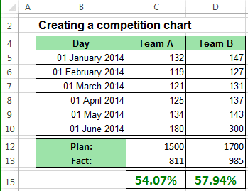
Creating a chart with dynamic labels - Microsoft Excel 2013
VBA to change data label in a chart - Compatibility btw ... It seems that Excel 2010 and 2013 work differently regarding to number format code in Macros. Due my limited access to Excel 2010, the solution was to duplicate the charts, change the labels as necessary and then switch the macro to show only the charts with the millions/thousands labels.
How to Add Data Labels in Excel - Excelchat | Excelchat
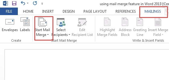
How to Print Labels from Excel - Lifewire Choose Start Mail Merge > Labels . Choose the brand in the Label Vendors box and then choose the product number, which is listed on the label package. You can also select New Label if you want to enter custom label dimensions. Click OK when you are ready to proceed. Connect the Worksheet to the Labels

Enable or Disable Excel Data Labels at the click of a button - How To - PakAccountants.com
Values From Cell: Missing Data Labels Option in Excel 2013? When a chart created in 2013 using the "Values from Cell" data label option is opened with any earlier version of Excel, the data labels will show as " [CELLRANGE]". If you want to ensure that data labels survive different generations of Excel, you need to revert to the old technique: Insert data labels Edit each individual data label

Add or remove data labels in a chart Right-click the data series or data label to display more data for, and then click Format Data Labels. Click Label Options and under Label Contains, select the Values From Cells checkbox. When the Data Label Range dialog box appears, go back to the spreadsheet and select the range for which you want the cell values to display as data labels.
Enable or Disable Excel Data Labels at the click of a button - How To - PakAccountants.com
How to add or move data labels in Excel chart? To add or move data labels in a chart, you can do as below steps: In Excel 2013 or 2016. 1. Click the chart to show the Chart Elements button . 2. Then click the Chart Elements, and check Data Labels, then you can click the arrow to choose an option about the data labels in the sub menu. See screenshot: In Excel 2010 or 2007

How to insert data labels to a Pie chart in Excel 2013 - YouTube
Adding rich data labels to charts in Excel 2013 ... You can do this by adjusting the zoom control on the bottom right corner of Excel's chrome. Then, select the value in the data label and hit the right-arrow key on your keyboard. The story behind the data in our example is that the temperature increased significantly on Wednesday and that appeared to help drive up business at the lemonade stand.

Charting in Excel - Adding Data Labels - YouTube
Excel 2013 - Line Chart Data Labels - Data Callout submenu ... In one of them I can see the Data Callout submenu which allows me to specific content for data labels to appear at specific points on the line-graph. The "label options/label contains" area in the formatting box then includes a "value from cells" tickbox that allows me specify that the values that come from a specific excel cell range.
How to use Mail Merge feature in Word 2013 | Tutorials Tree: Learn Photoshop, Excel, Word ...
Creating a chart with dynamic labels - Microsoft Excel 2013 Excel 2013 365 2016 This tip shows how to create dynamically updated chart labels that depend on value or other cells. The trick of this chart is to show data from specific cells in the chart labels.

SQL & BI Learning: Pie Chart with data labels outside in ssrs
Custom Data Labels with Colors and Symbols in Excel Charts ... To apply custom format on data labels inside charts via custom number formatting, the data labels must be based on values. You have several options like series name, value from cells, category name. But it has to be values otherwise colors won't appear. Symbols issue is quite beyond me.

Australia - Geographic State Heat Map - Excel Template - INDZARA
How to Add Data Labels in Excel - Excelchat | Excelchat How to Add Data Labels In Excel 2013 And Later Versions In Excel 2013 and the later versions we need to do the followings; Click anywhere in the chart area to display the Chart Elements button Figure 5. Chart Elements Button Click the Chart Elements button > Select the Data Labels, then click the Arrow to choose the data labels position. Figure 6.

How-to Use Data Labels from a Range in an Excel Chart - Excel Dashboard Templates
How to Create and Label a Pie Chart in Excel 2013 : 8 ... Step 8: Label the Chart. Check the "Data Labels" square and the labels will appear on the pie chart. Congratulations, you have successfully created a labeled pie chart. Note: If you want to re-position the labels, hover your cursor over the "Data Labels" option and click on the small, black triangle that appears next to it.
Adding and editing data labels Microsoft Excel 2016 Microsoft Excel 2016 - YouTube
Excel Tips n Tricks -Tip 8 (Applying Chart Data Labels ... Click on the plus symbol, the first icon, and check "Data Labels". Now you will see them added to your chart. You can also click on the right arrow on "Data Labels" and select where you want the data labels to be aligned, in other words center, right, top, bottom and so on. Picture 4 4. I modified the chart and axis titles to look good.
Advanced Excel - Краткое руководство - CoderLessons.com
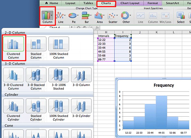
Create a Histogram Graph in Excel
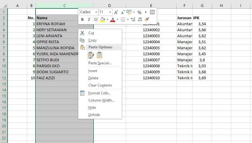
Cara Membuat Kolom Custom Di Excel Dengan Mudah
Post a Comment for "44 data labels excel 2013"